Clase teórica Semana 10

Autor/a

Marylia Cruz

Fecha de publicación

26 de mayo de 2025

peliculas=c("driver","mike7","destinofinal","frozen","flow")
año=c(2011,2025,2000,2013,2024)
genero=c("accion","cienciafiction","terror","animacion","animacion")

data=data.frame(peliculas,año,genero)

library(rio)
#export(data,"peliculas.csv") #csv delimitado por comas
#export(data,"peliculas.xlsx") #xlsx para guarr un archivo en excel

data2=import("data/Base_Peliculas_Disney-2.sav")

names(data2)

[1] "titulo_pelicula"          "fecha"                   
[3] "antigüedad"               "genero"                  
[5] "mpaa_rating"              "total_gross"             
[7] "inflation_adjusted_gross" "genero2"                 
[9] "mpaa_rating2"

names(data2)[6] <- "ingresos"

tail(data2)

str(data2)

'data.frame':   579 obs. of  9 variables:
 $ titulo_pelicula         : chr  "Snow White and the Seven Dwarfs" "Pinocchio" "Fantasia" "Song of the South" ...
  ..- attr(*, "format.spss")= chr "A40"
  ..- attr(*, "display_width")= int 40
 $ fecha                   : Date, format: "1937-12-21" "1940-02-09" ...
 $ antigüedad              : num  84.9 82.8 82 76 72.7 ...
  ..- attr(*, "format.spss")= chr "F18.15"
  ..- attr(*, "display_width")= int 16
 $ genero                  : chr  "Musical" "Adventure" "Musical" "Adventure" ...
  ..- attr(*, "format.spss")= chr "A19"
  ..- attr(*, "display_width")= int 19
 $ mpaa_rating             : chr  "G" "G" "G" "G" ...
  ..- attr(*, "format.spss")= chr "A9"
  ..- attr(*, "display_width")= int 9
 $ ingresos                : num  1.85e+08 8.43e+07 8.33e+07 6.50e+07 8.50e+07 ...
  ..- attr(*, "format.spss")= chr "F12.10"
  ..- attr(*, "display_width")= int 12
 $ inflation_adjusted_gross: num  5.23e+09 2.19e+09 2.19e+09 1.08e+09 9.21e+08 ...
  ..- attr(*, "format.spss")= chr "F13.11"
  ..- attr(*, "display_width")= int 12
 $ genero2                 : num  10 3 10 3 8 3 8 8 5 5 ...
  ..- attr(*, "format.spss")= chr "F2.0"
  ..- attr(*, "display_width")= int 9
  ..- attr(*, "labels")= Named num [1:12] 2 3 4 5 6 7 8 9 10 11 ...
  .. ..- attr(*, "names")= chr [1:12] "Action" "Adventure" "Black Comedy" "Comedy" ...
 $ mpaa_rating2            : num  5 5 5 5 5 NA 5 NA 5 NA ...
  ..- attr(*, "format.spss")= chr "F1.0"
  ..- attr(*, "display_width")= int 14
  ..- attr(*, "labels")= Named num [1:5] 1 2 3 4 5
  .. ..- attr(*, "names")= chr [1:5] "R" "PG-13" "PG" "Not Rated" ...

table(data2$genero)


                                 Action           Adventure        Black Comedy 
                 17                  40                 129                   3 
             Comedy Concert/Performance         Documentary               Drama 
                182                   2                  16                 114 
             Horror             Musical     Romantic Comedy   Thriller/Suspense 
                  6                  16                  23                  24 
            Western 
                  7

library(dplyr)


Attaching package: 'dplyr'

The following objects are masked from 'package:stats':

    filter, lag

The following objects are masked from 'package:base':

    intersect, setdiff, setequal, union

tabla_frecuencia = data2 %>%
  count(genero) %>% 
  filter(!genero %in% "") #removemos valores perdidos
tabla_frecuencia

tabla_porcentajes= data2 %>%
  count(genero) %>% 
  filter(!genero %in% "") %>% #removemos valores perdidos
  mutate(porcentaje = n / sum(n) * 100)  # Calculamos el porcentaje
tabla_porcentajes

library(ggplot2)
ggplot(tabla_porcentajes, aes(x=genero,y=porcentaje, fill=genero))+
  geom_bar(stat = "identity")+
    coord_flip()+
  labs(title = "Gráfico de barras de porcentaje de peliculas por Genero",
       x = "Genero",
       y = "Porcentaje") +
  theme_minimal() +  # Tema minimalista
  scale_fill_brewer(palette = "Set3")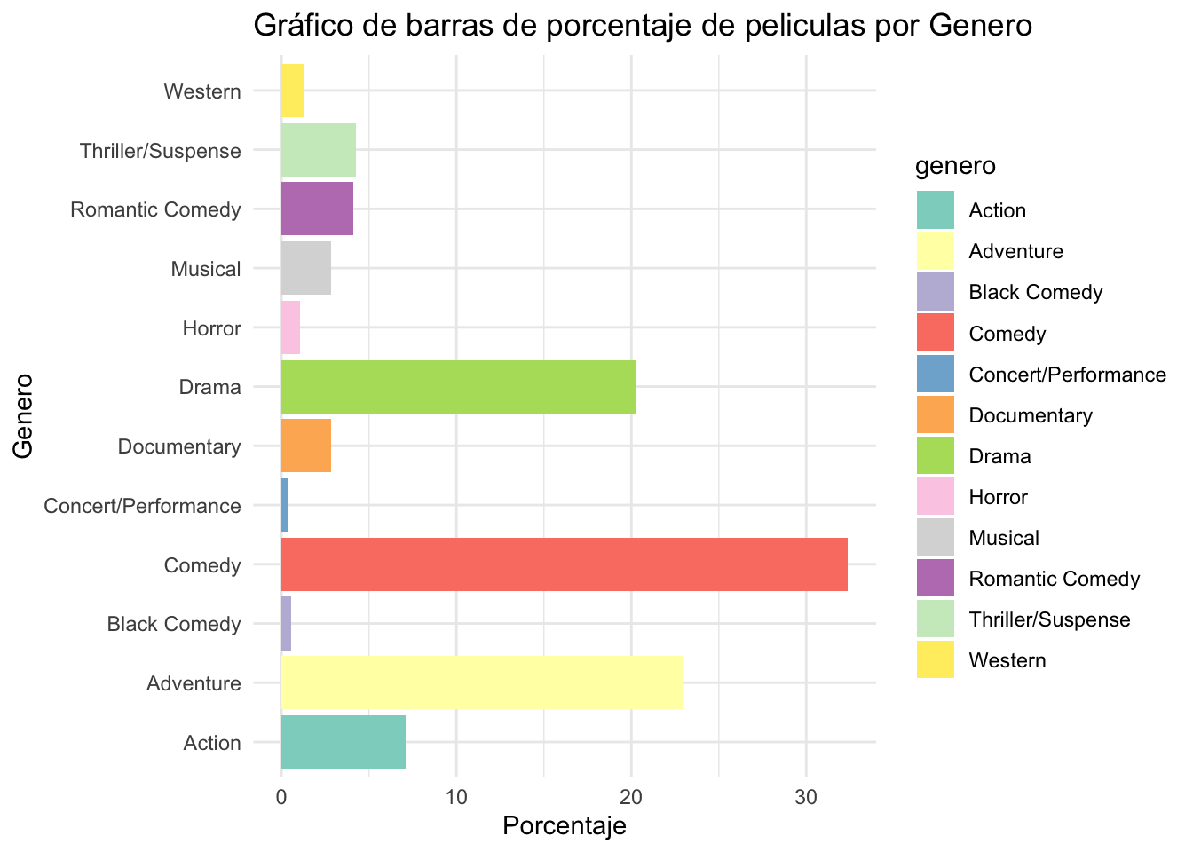

tabla_porcentajes2= data2 %>%
  count(mpaa_rating) %>%
  filter(!mpaa_rating %in% "") %>% #removemos valores perdidos
  mutate(porcentaje = n / sum(n) * 100)  # Calculamos el porcentaje
tabla_porcentajes2

library(ggplot2)
ggplot(tabla_porcentajes2, aes(x=mpaa_rating,y=porcentaje, fill=mpaa_rating))+
  geom_bar(stat = "identity")+
    coord_flip()+
  labs(title = "Gráfico de barras de porcentaje de peliculas por MPAA",
       x = "MPAA",
       y = "Porcentaje") +
  theme_minimal() +  # Tema minimalista
  scale_fill_brewer(palette = "Set3")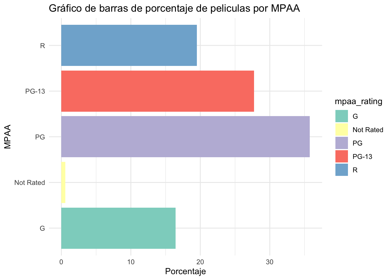

mean(data2$ingresos)

[1] 64701789

summary(data2$ingresos)

     Min.   1st Qu.    Median      Mean   3rd Qu.      Max. 
        0  12788864  30702446  64701789  75709033 936662225

data2$antigüedad=as.numeric(data2$antigüedad)

summary(data2$antigüedad)

   Min. 1st Qu.  Median    Mean 3rd Qu.    Max. 
  5.849  16.714  24.145  24.297  29.582  84.890

ggplot(data2,aes(x=antigüedad))+
  geom_histogram()

`stat_bin()` using `bins = 30`. Pick better value with `binwidth`.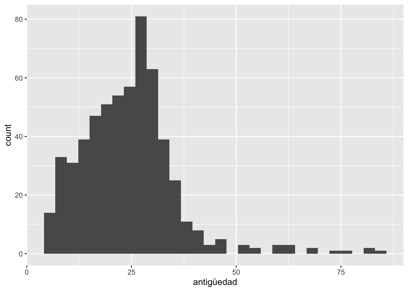

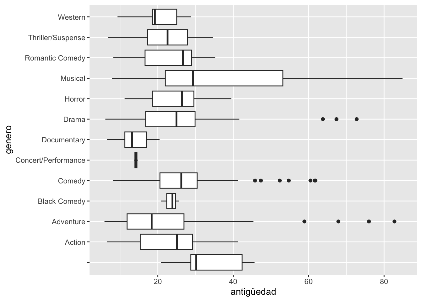
ggplot(data2,aes(y=antigüedad,x=genero))+
  geom_boxplot() +
  coord_flip()