Clase teórica Semana 13

pruebas bivariadas

Abrir la base de datos

library(rio)
data=import("data/Data_ejemplo_comunica.xlsx")

names(data)

[1] "N"                               "Nivel de procastinacion"        
[3] "RedSocial"                       "Tiempo en redes sociales"       
[5] "Le gusta Leer"                   "Numero de interacciones diarias"
[7] "Numero de Seguidores"           

Prueba T de student

t.test(`Tiempo en redes sociales` ~ `Le gusta Leer`, data = data)

    Welch Two Sample t-test

data:  Tiempo en redes sociales by Le gusta Leer
t = 20.31, df = 170.27, p-value < 2.2e-16
alternative hypothesis: true difference in means between group NO and group SI is not equal to 0
95 percent confidence interval:
 160.4916 195.0484
sample estimates:
mean in group NO mean in group SI 
          277.61            99.84 

library(dplyr)

Attaching package: 'dplyr'

The following objects are masked from 'package:stats':

    filter, lag

The following objects are masked from 'package:base':

    intersect, setdiff, setequal, union

library(lsr)
tabla=data%>%
  group_by(`Le gusta Leer`)%>%
  summarise(
  promedio=mean(`Tiempo en redes sociales`),
  linferior=ciMean(`Tiempo en redes sociales`)[1],
    lsuperior=ciMean(`Tiempo en redes sociales`)[2]
)

tabla

Gráfico de prueba T

library(ggplot2)
ggplot(tabla, aes(x = `Le gusta Leer`, y = promedio)) +
  geom_errorbar(aes(ymin = linferior, ymax = lsuperior), width = 0.2) +
  labs(x = "Le gusta leer o no", y = "Media ± IC 95%") +
  theme_minimal()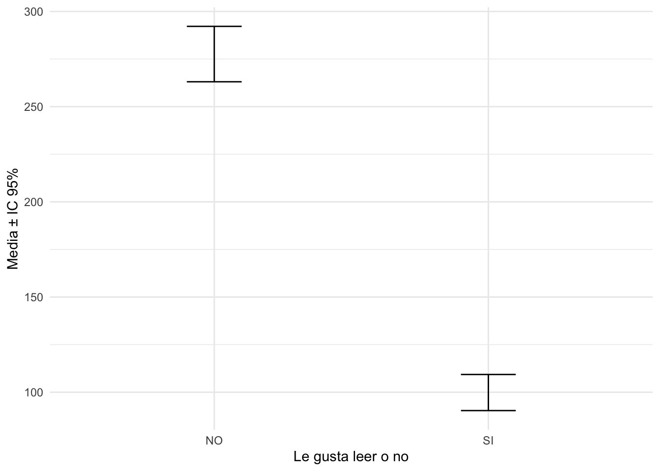

Prueba Anova

anova=aov(`Numero de Seguidores` ~`RedSocial`,data=data)

summary(anova)

             Df  Sum Sq Mean Sq F value Pr(>F)    
RedSocial     2 1470386  735193     153 <2e-16 ***
Residuals   197  946705    4806                   
---
Signif. codes:  0 '***' 0.001 '**' 0.01 '*' 0.05 '.' 0.1 ' ' 1

Gráfico de prueba Anova

library(dplyr)
library(lsr)
tabla=data%>%
  group_by(`RedSocial`)%>%
  summarise(
  promedio=mean(`Numero de Seguidores`),
  linferior=ciMean(`Numero de Seguidores`)[1],
    lsuperior=ciMean(`Numero de Seguidores`)[2]
  
)

tabla

library(ggplot2)
ggplot(tabla, aes(x = RedSocial, y = promedio)) +
  geom_errorbar(aes(ymin = linferior, ymax = lsuperior), width = 0.2) +
  labs(x = "Grupo", y = "Media ± IC 95%") +
  theme_minimal()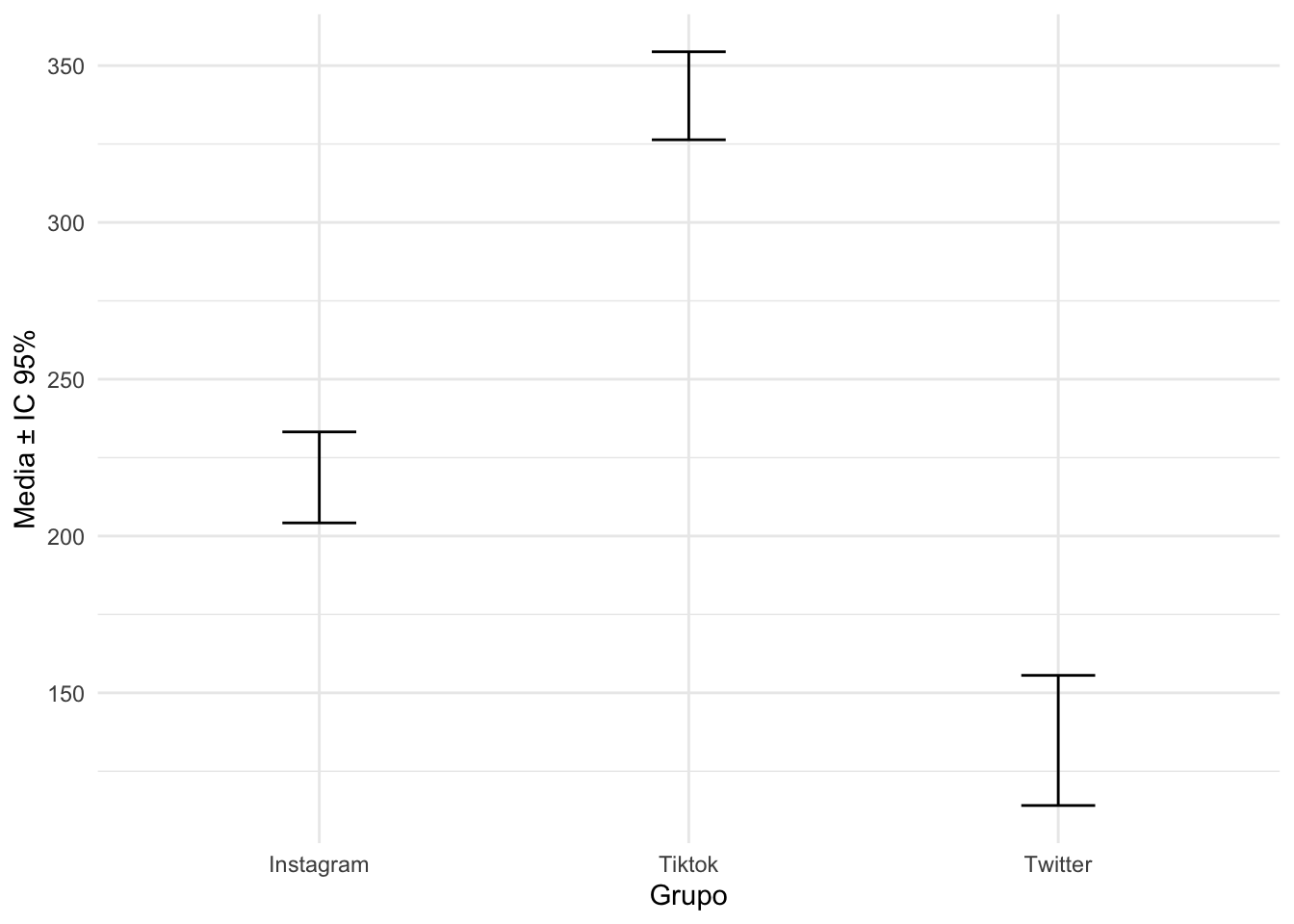

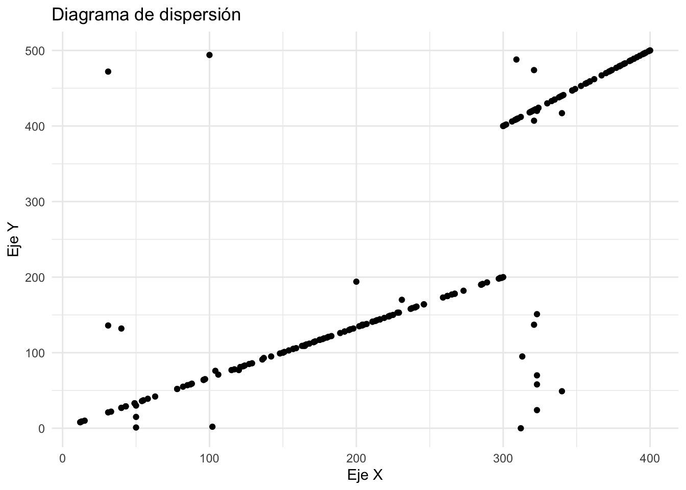
Prueba de Correlación

cor.test(data$`Numero de Seguidores`,data$`Numero de interacciones diarias`)

    Pearson's product-moment correlation

data:  data$`Numero de Seguidores` and data$`Numero de interacciones diarias`
t = 20.181, df = 198, p-value < 2.2e-16
alternative hypothesis: true correlation is not equal to 0
95 percent confidence interval:
 0.7690670 0.8610325
sample estimates:
      cor 
0.8202829 

Gráfico de dispersión

library(ggplot2)

ggplot(data, aes(x = `Numero de Seguidores`, y = `Numero de interacciones diarias`)) +
  geom_point() +
  labs(title = "Diagrama de dispersión", x = "Eje X", y = "Eje Y") +
  theme_minimal()