Clase teórica Semana 15

Repaso

Ejercicio de repaso

library(rio)
data2=import("youtube_data.csv")

names(data2)

 [1] "video_id"       "title"          "description"    "published_date"
 [5] "channel_id"     "channel_title"  "tags"           "category_id"   
 [9] "view_count"     "like_count"     "comment_count"  "duration"      
[13] "thumbnail"     

str(data2$view_count)

 num [1:600] 8962092 289626 81372201 21255964 2790436 ...

str(data2$like_count)

 num [1:600] 243350 3393 4178447 909386 44278 ...

Existe una relación entre el número de vistas y el número de likes?

cor.test(data2$view_count,data2$like_count)

    Pearson's product-moment correlation

data:  data2$view_count and data2$like_count
t = 23.975, df = 598, p-value < 2.2e-16
alternative hypothesis: true correlation is not equal to 0
95 percent confidence interval:
 0.6568404 0.7387255
sample estimates:
      cor 
0.7000773 

Gráfico de dispersión

library(ggplot2)

ggplot(data2, aes(x = view_count, y = like_count)) +
  geom_point() +
  labs(title = "Diagrama de dispersión", x = "Eje X", y = "Eje Y") +
  theme_minimal()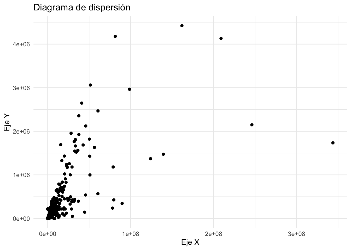

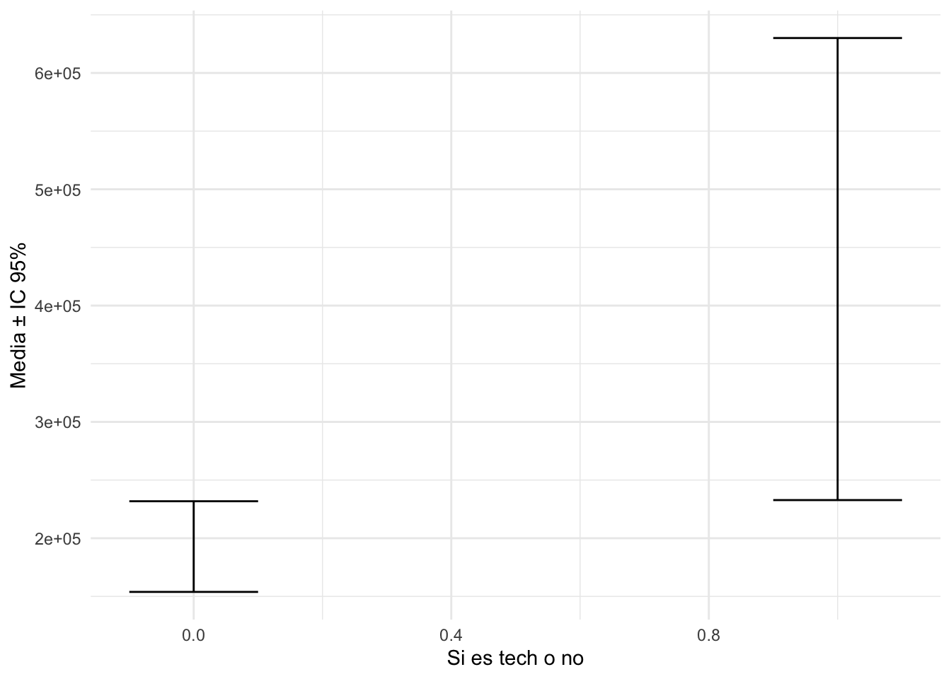
Calculamos la variable es_tech por si se repite un patrón en tags

data2$es_tech=ifelse(grepl("'tech'",data2$tags),1,0)

table(data2$es_tech)

  0   1 
538  62 

Existe una diferente de medias del número de likes entre los videos que pertenecen al grupo tech o no ?

t.test(like_count~es_tech,data=data2)

    Welch Two Sample t-test

data:  like_count by es_tech
t = -2.3555, df = 65.953, p-value = 0.02148
alternative hypothesis: true difference in means between group 0 and group 1 is not equal to 0
95 percent confidence interval:
 -440840.7  -36354.8
sample estimates:
mean in group 0 mean in group 1 
       192809.5        431407.3 

Gráfico de barras de error

library(lsr)
library(dplyr)

Attaching package: 'dplyr'

The following objects are masked from 'package:stats':

    filter, lag

The following objects are masked from 'package:base':

    intersect, setdiff, setequal, union

tabla=data2%>%
  group_by(es_tech)%>%
  summarise(
  promedio=mean(like_count),
  linferior=ciMean(like_count)[1],
    lsuperior=ciMean(like_count)[2]
)

tabla

library(ggplot2)
ggplot(tabla, aes(x = es_tech, y = promedio)) +
  geom_errorbar(aes(ymin = linferior, ymax = lsuperior), width = 0.2) +
  labs(x = "Si es tech o no", y = "Media ± IC 95%") +
  theme_minimal()